Problem Statement

Consider the following problem: “You launch a water balloon from ground level at an initial speed at an angle θ above the horizontal. Determine the balloon's velocity at different points in its trajectory, specifically the vertical component of velocity as a function of time, when considering both upward and downward directions.” — Savov (2016, p. 238)

This classic kinematics problem, which incorporates elements of calculus, will be solved both manually and through Python programming. I will start by deriving the motion equations from a sketch I created and subsequently plot the velocities for various θ values.

Kinematics Equations

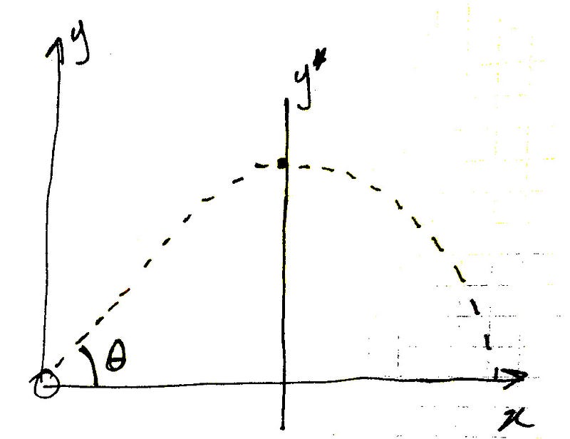
To visualize the problem, refer to Figure 1, which illustrates the scenario described:

In classical physics, the connection between force, acceleration, velocity, and displacement is expressed by the following equation:

This equation separates the forces acting on an object (left side) from the object's motion (right side). In this case, I will focus on defining acceleration based on this graph, rather than analyzing the forces affecting it.

The water balloon is projected from the origin at angle θ. When analyzing the motion concerning the vertical axis, the sine function comes into play. Equation 2.1 provides the acceleration function for the water balloon:

Here, -g represents the gravitational acceleration in kinematic equations. Incorporating this, Equation 2.2 is formulated:

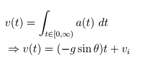
From the initial equation, we recognize that an object's acceleration is the derivative of its velocity, while velocity is the derivative of its displacement. Given that I only have the acceleration, I will apply anti-derivatives to derive both the velocity and displacement functions from Equation 2.2. Equation 3.1 illustrates the resulting velocity function:

Similarly, the displacement function can be derived from the velocity function, represented by Equation 3.2:

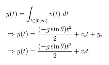
I omitted the initial vertical position since the balloon is launched from the ground (i.e., y₀ = 0). The problem also queries the kinematic equations under an unusual scenario where gravity acts upward. These equations can be derived by reversing the signs of the gravitational and initial velocity coefficients in Equations 3.1 and 3.2.

To verify the results, I used the Sympy Live Shell, as shown in Figure 2:

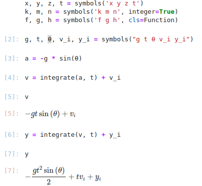
It's important to note that Sympy does not automatically include the constant of integration, so I had to add that manually. Additionally, I avoided specifying concrete units (like meters or seconds) to simplify the problem as an abstract mathematical exercise.

Visualisation

To visualize the derived kinematics equations, I employed Python and Matplotlib. I began by launching Jupyter Notebook and importing the necessary libraries:

import math

import numpy as np

import matplotlib.pyplot as plt

Next, I implemented the displacement function I derived:

def y(t, θ):

y = -9.81 * math.sin(math.radians(θ))

y = y * t**2 / 2.0 + 10 * t

return y

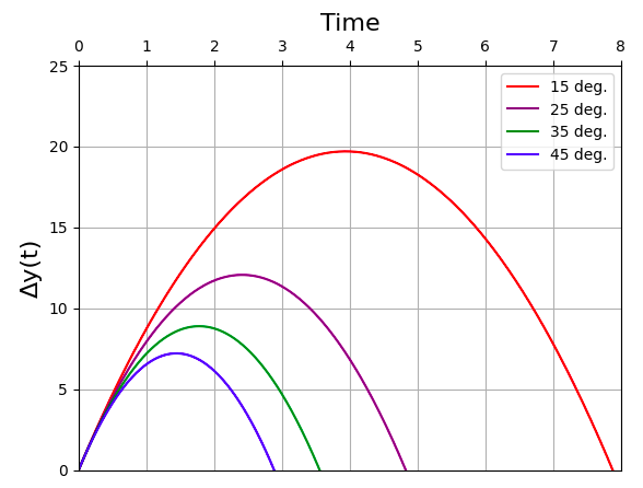
Using a gravitational constant of 9.81 and an initial velocity of 10, I set the plotting range and defined angles for visualization:

R = np.arange(0, 10, 0.01)

angles = [

[15, "red"],

[25, "purple"],

[35, "green"],

[45, "blue"]

]

I then set up the plot and visualized each angle:

plt.figure()

plt.rcParams['xtick.bottom'] = plt.rcParams['xtick.labelbottom'] = False

plt.rcParams['xtick.top'] = plt.rcParams['xtick.labeltop'] = True

for k in angles:

plt.plot(R, [y(t, k[0]) for t in R], color=k[1], label=str(k[0]) + " deg.")

plt.legend()

plt.grid()

plt.title("Water Balloon Trajectory Over Time", fontsize=16)

plt.ylabel("Vertical Position y(t)", fontsize=16)

plt.ylim(0, 25)

plt.xlim(0, 8)

plt.show()

Figure 3 illustrates the resulting kinematics plot:

References

Savov, I. (2016). No Bullshit Guide to Math & Physics. Minireference Publishing.